|
|
Post by finiteparts on Mar 21, 2015 13:21:43 GMT -5
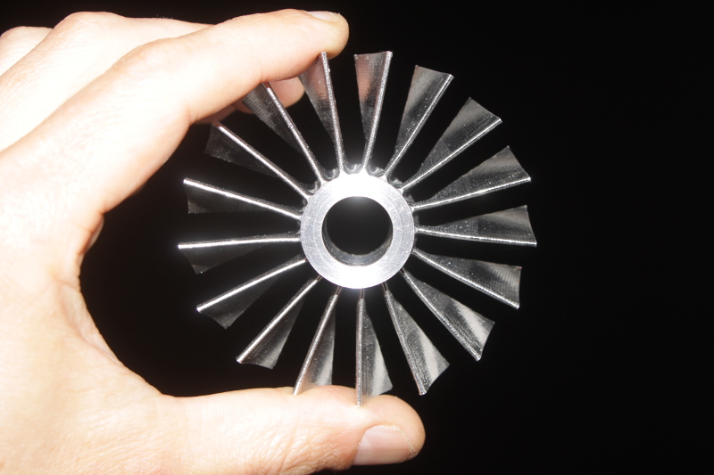
John, I finally got around to measuring that Rotax/Lucas rotor. Sorry for the delay. Hopefully I got all the measurements you wanted, but if not, let me know what you need. You can see the compressor impeller vanes are exactly the same height as the diffuser passage, 0.275 inch.   ~ Chris |
|
|
|
Post by racket on Mar 21, 2015 16:40:01 GMT -5
Hi Chris
Thanks for the numbers , it adds to the "knowledge store" :-)
I can do some reverse engineering on them to get an idea of whats happening
Cheers
John
|
|
|
|
Post by finiteparts on Apr 26, 2015 13:37:40 GMT -5
I have been working recently on programming the component matching equations into my "design software" and I ran across something that I thought was pretty interesting. In a simplified sense the matching of a turbocharger can be reduced to two primary equations. These are given in several sources, but I will cite them from Baines, "Fundamental of Turbocharging". When these equations are plotted, you get a plot of the required turbine expansion ratio for a given compressor pressure ratio and a plot of the corrected mass flow through a turbine vs the expansion ratio. Here is the plot from what Baines refers to as the "first turbocharger equation" assuming: 1. compressor system efficiency of 78% 2. turbine system efficiency of 75% 3. 95% mechanical efficiency 4. Mass flow addition of 1% in the combustor 5. Constant ratio of specific heats for the cold side 6. Constant ratio of specific heats for the hot side 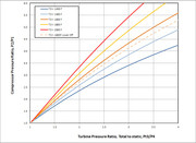 So if we look at this plot, it gives the behavior we would expect. I've marked up a version of this to show the trends...  Let's say we are trying to get a pressure ratio from the compressor system of 3, which I have marked as the black horizontal line. As we move over we see that we intersect a group of curves. These are curves of constant temperature ratio, specifically, the total gas temperature entering the turbine system over the ambient inlet temperature. From these curves, we can see that as the turbine inlet temperature is increased, (temp ratio increases since ambient is fixed), we need less gas expansion through the turbine stage. But, we know that our uncooled turbines can only support a certain gas temperature before we experience high nickel emissions...so let use 1600 F as the upper temperature limit. The 1600 F condition is shown as sort of a brown curve in the middle of all the curves. Now, if we reduce the turbine efficiency by 3% and everything else stays the same, we get the curve show just below it in the lighter brown dashed curve. If we follow that down to find the required turbine expansion ratio, we see that we now have to use more pressure drop through the turbine to make the power required by the compressor to get a PR =3. But, what if we don't have that much pressure drop available because we took a big loss in the combustor or in the ducting? We can see that if we had for example only enough pressure for a 2:1 expansion in the turbine, then our gas temperature would have to be above our 1600 F limit to provide that power to the compressor. The turbine would require a inlet temperature of almost 1800 F to keep up with the compressor power requirements. These lines of constant temperature ratio can be plotted on a standard compressor map (with some work and assuming the turbine inlet is choked) and give a plot similar to this, 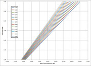 which shows them in corrected mass flow values (or as many turbocharger manufacturers state, mass flow parameter, MFP). Since the assumption of the turbine being choked, we can see that these curves would be incorrect at lower pressure ratios, where they just turn and curve towards the PR=1 and corrected mass flow = 0 point. Converting these to the current ambient pressure and temperature yields lines of mass flow rate... 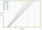 So now we have an idea of the mass flow rates that we have entering the turbine, so we can convert the mass flow rate into a corrected mass flow rate and see where we fall on the plot of what is termed the "second turbocharger equation". I have it plotted here with several values of effective throat area.. 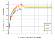 This is were the problem comes up. If you look at the plot, it looks like we would expect, the corrected mass flow rate chokes at some expansion ratio and the corrected mass flow rate for larger throats is larger. But, if you look close, the critical pressure ratio is the same for all the curves. At a pressure ratio of around 1.78 all the throats choke. Now this is exactly what we would expect from one-dimensional compressible flow...that there is a critical pressure ratio which is only a function of the ratios of specific heats (gamma) and for this gamma it is around 1.78. So what's the problem? The problem is this... 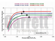 If you look at where each of the curves shows the corrected flow chokes, it is not at around 1.78 that the one-dimensional compressible flow predicts! There are other maps out there that have critical pressure ratios near 3:1... So what's the problem here? The problem is our assumptions. We are using the one-dimensional compressible flow equations which assume ideal, isentropic flow! Isentropic means that there is constant entropy...or in this case, it is worded better as NO change in entropy. Entropy is a fancy word for irreversible losses...these are like losses due to friction, turbulence, losses due to scrubbing friction of the flow, etc. Thus, using the one-D equations, as the flow goes through the turbine there is no entropy generated under this assumption! Really?! What?!!! It took quite a bit of searching, but I found a good reference that discussed the issue (Hesse and Mumford's "Jet Propulsion for Aerospace Applications"). So a quick look at a enthalpy - entropy (H-S) diagram may help...by the way, again, enthalpy is the internal energy of the flow and the entropy is the amount of unrecoverable losses in the flow. 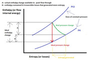 So, if we are expanding from the total pressure at the inlet, Pt3, down to the static pressure at the outlet, P4 and doing it isentropically (constant entropy), we would move along the red vertical line since the entropy would not change. Also, as a point of information, if we did this expansion isentropically, the total pressure at the exit would not have changed...the total pressure only changes when there are losses or heat addition/subtraction or mechanical work has been done to or by the flow. But, since we live in the real world, there are always irreversible losses...so we will generate some entropy as we go through the turbine system and reduce the gas pressure along the green curve path. So we are generating entropy and because of this some of the flows internal energy is consumed by these sources of loss such that we have less flow internal energy to get through the turbine system. This means that the pressure ratio required to push the corrected mass flow through the turbine must go up and thus not follow the predictions given by the one-dimensional ideal flow compressible equations. So if we used those to size our nozzle guide vane throats, we would have under-predicted the corrected mass flow rate for a given pressure ratio. So, Hesse and Mumford provide an equation for the critical pressure ratio of a nozzle with an efficiency term (the turbine system is modeled as a nozzle by Baines and others). The use of this allows modification of the critical pressure to match the curves provided by the vendors turbine maps. I have not found a corrected mass flow rate equation which incorporates this real world effect and I am trying to derive that equation from the nozzle friction parameter equations provided in Hesse and Mumford's work. Additionally, Grietzer, et. al. provide some nice insight to real world effects in their work "Internal Flows, Concepts and Applications". I am still working through the chapter on compressible internal flows that covers a vast array of potential sources of discrepancies between the ideal, fritionless, isentropic case and more real world applications. The cursory look appears that there may be noticeable effects due to friction, heat transfer, asymmetric swirling flows among others. Now, just to clarify, my design software uses iterative loops to solve for unknown parameters and then calculates the vectors due to the local conditions and I am not trying to use the above equations as a means to calculate any of my conditions...I was only playing with them as a curiosity when I notice the choked flow issue. So that made me concerned because my program uses the one-dimensional compressible equations with the assumption that the isentropic case was close enough...but after playing with the above equations, I feel that assumption is a potential source of large errors. I thought that I would share this information in case anyone else is relying on these same equations for their design. Good luck! Chris |
|
|
|
Post by finiteparts on Apr 26, 2015 14:52:45 GMT -5
On a similar note, I forgot to highlight the use of corrected mass flow in the above post. I feel that some people out there may be getting the wrong idea about choked flows and reading maps. First, if we look at this turbine map, we see that the bottom axis is not mass flow, but a mass flow parameter... 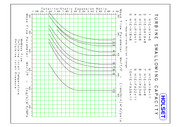 Maps are corrected so that different entrance conditions can be represented on a single map...if they didn't do this, the map for a 1100 F TIT would be different to the map of a 1600 F TIT. The same thing holds for the compressor maps. So in the above Holset map, to get the actual mass flow, you have to multiply it by the inlet pressure and divide by the square root of the temperature. If you read right off the map you will have an incorrect value unless you just so happen to be at the reference conditions. For example, if I look at the Garrett turbine map I had in the last post and take the A/R = 1.06 case, it would be easy to say that the choked mass flow is 35 lbm/min. I would think that I have an upper limit of 35 lbm/min that I could push through the engine no matter what I do, I can't get the engine mass flow greater than 35 lbm/min. WRONG!!! If that was the case, then larger gas turbines wouldn't be able to run up to the high pressure ratios that they do. Most commercial engines operate the majority of their existence at conditions of choked turbine nozzles and choked exhaust nozzles (double choked). If they have power turbines, the stages of the power turbines often act as being fully choked even though they might not be. So I have a complaint with Garrett maps...they do not state what they have been corrected too. Holset does a nice job...Borg Warner does sometimes... The Garrett map shown above is almost worthless for us because I cannot get the actual mass flow from that map without knowing what they "corrected" it to. My guess is that there is a SAE spec out there that tells us, but for now I will just switch over to the Holset map. So let's look at turbine housing #5....which chokes at a MFP = 42 kg/s*sqrt(K)/MPa. Plugging in a PR = 2.6 and an inlet temperature of 1600 F (1144 K) we get 0.3272 kg/s (43.28 lbm/min). Let's say that I move up on the choke line to a higher pressure ratio...it looks like it should be the same mass flow from the plot, right? Nope...At a pressure ratio of 2.8, I get for the same inlet temperature, a mass flow rate of 0.3529 kg/s (46.61 lbm/min). So why can I get more mass flow rate through the engine if the turbine is choked? Choked means that the velocity at the throat has reached the speed of sound for the given inlet conditions. So mass flow is density * velocity * area. Area doesn't change...but the velocity and density do. The critical velocity (speed of sound) changes as a function of temperature (= sqrt(gamma*R*T)), so even the velocity doesn't stay fixed. When the throat chokes, the conditions downstream don't do anything to change the flowrate through the throat. But the conditions upstream can effect the conditions at the throat and thus can change the mass flow rate at choked conditions. By increasing the pressure upstream, we saw from the above example that the swallowing capacity of the throat was increased. If we just increased the temperature, the swallowing capacity of the throat would be reduced. But, in an engine, we can't just increase temperature without effecting everything upstream and changing the pressure too. In a gas turbine engine, the only knob we have to control is usually the fuel flow rate. Increase fuel flow and get a hotter combustor condition giving us a drop in gas density...this increases the amount of pushing the compressor has to do to get that mass flow rate through the same area and thus the pressure ratio rises. If we plot them as separate effects, the results look like this...  So be careful when looking at maps...the corrected numbers need to be calculated and not just assumed to be the same. Also, hopefully now you can say how an engine can run and be controlled when it's NGVs are fully choked. Good luck! Chris |
|
|
|
Post by finiteparts on Apr 26, 2015 15:37:40 GMT -5
In my ever expanding collection of nifty turbomachinery bits, I have recently acquired some nice ceramic turbocharger turbines. The ceramic turbines have been an interest of mine for many years. Ceramics offer some nice properties, but they have a nasty propensity for brittle fracture that has made many engineers scared of them. I have a folder or two of the work that Toyota, GM, Garrett, Nissan etc did with Kyocera and others to make these production ready. I have a Nissan turbo with ball bearing center cartridge and a ceramic turbine wheel that I have been toying with making into a small test engine. So here are the recent Garrett acquisitions...apparently a engineer from Garrett retired (and maybe passed away?) and someone was selling his desk art off on eBay...so I picked up these beauties!  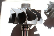 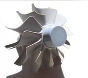  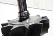 Then I also have two of what I think are Toyota turbine wheels. Notice that even though these are both silicon nitride, they have vastly different appearances. I also have a Toyota CT-26 turbine that is a beautiful gray appearance...I'll have to bring that home from work to photograph it. I use it at work to challenge other engineers preconceived notions of ceramic parts. A salesman I met for a ceramic company had a ceramic hammer and let you drive nails in a board all day with it. 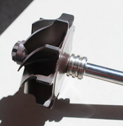 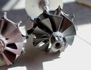 Notice the difference in how the ceramic wheel is held into the shaft. Since the thermal expansion coefficients are so different, there is a lot of engineering involved in that connection! Enjoy! Chris |
|
|
|
Post by racket on Apr 26, 2015 16:49:26 GMT -5
Hi Chris
Now that was a handful to digest :-)
From a Garrett Publication
Turbine Correct Flow =
Actual Flow X the square root of ( Gas Temperature + 460) /519
--------------------------------------------------------------------
(Barometric Pressure + Exhaust Manifold Pressure) /14.7
Turbine expansion ratio =
Exhaust manifold pressure + atmospheric pressure
------------------------------------------------------
Turbine outlet pressure + atmospheric pressure
This equation is a bit "suspect" as the "outlet pressure" is assumed as static or is it total , they don't say , only that its 1 psi in the worked example.
The subject does get complicated , especially when we don't generally have any idea what our compressor and turbine efficiencies are , the limited number of maps available means good old "trial and error" methods end up being the only alternative .
Some rough general assumptions can often be used to get in the ball park , but its still going to need testing to produce data that can then be used to put into the equations.
Thanks for all the work in getting this info up here , its much appreciated :-)
Cheers
John
|
|
|
|
Post by finiteparts on Apr 27, 2015 21:19:48 GMT -5
Thanks for that info John. I would have never guessed that they would have corrected it to ISO day conditions (59 F and 14.696 psi)...I get that for the compressor side, but the turbine side is interesting. Is this a document that they have online? I would guess that they also use the standard total to static pressure ratio...but like you said, without them stating it, how do we know? I don't know how I missed it, but I pulled out my copy of Saad's compressible flow book and there is a nice section on nozzle and diffuser efficiency. This is the book that I provided a link to in a previous post... jetandturbineowners.proboards.com/post/11013Go to page 123...if I had seen this it would have saved me the time of drawing out that figure! I am still trying to see if I can modify the equations for the mass flow vs pressure ratio to include the "efficiency" term, to see if I can match the curves for other housings. Especially, since I can't seem to find this worked out anywhere...now it is just a curiosity and a challenge! ~ Chris |
|
|
|
Post by racket on Apr 27, 2015 21:59:43 GMT -5
Hi Chris
I've had the info for years , it was originally on a Garrett Tech Info document, Page 24 , but I've never been able to find it online in recent years.
Some of my very old Garrett comp maps had the "Correction Factors " printed on them, heres whats on a TV81 map, Circa 1980
Corrected Mass Flow .........
W X sq root (inlet total temp /545)
--------------------------------------
Comp inlet total pressure,inches Hg Abs/28.4
Rpm correction factor ................
N
--------------------------------------
comp inlet total temp degrees R/545
Cheers
John
|
|
|
|
Post by finiteparts on May 22, 2015 17:02:19 GMT -5
So I mentioned that I was reading several papers from the guys over at Queen's College in Belfast and finally, I decided to type up the summaries of those. The first paper is: S.W.T. Spencer and D.W. Artt, "An experimental assessment of incidence losses in a radial inflow turbine rotor" Proceedings of the Institution of Mechanical Engineers, Part A: Journal of Power and Energy February 1, 1998 212: 43-53 pia.sagepub.com/content/212/1/43.full.pdf The authors tackle the rather challenging problem of determining the effect of flow incidence loss on the overall turbine performance. They begin by a review of the previous loss models out there, these include: 1. F.J.Wallace's "shock-loss" model that supposed that the sudden deflection of the flow into the rotor and its associated loss in kinetic energy, could be represented as reheat at constant pressure. Later (in other paper) the author showed that this was incorrect if he assumed a blockage due to the presence of the blade thickness. pme.sagepub.com/content/172/1/931 2. NASA work...these include works by: a. Futral and Wasserbauer - unable to find online resource b. Todd and Futral - "A FORTRAN 4 program to estimate the off-design performance of radial-inflow turbines" ntrs.nasa.gov/search.jsp?R=19690010475 c. Wasserbauer and Glassman - "FORTRAN program for predicting off-design performance of radial-inflow turbines" ntrs.nasa.gov/search.jsp?R=19750024045 3. Rodgers - "Meanline performance prediction for radial inflow turbines", VKI Lecture series 1987 - unable to find online resource The authors of the paper point out that there is a lack of published performance data to support these loss models and many of the older reports often have questionable data due to the assumptions they used to back out the losses from the measured data. Their experimental data is based on a 99.06 mm inlet diameter turbine, with a 64 trim. The turbine is a production turbocharger part (likely a Garrett, since they thank Allied Signal at the end of the paper) that has been trimmed to achieve a desired specific speed. The challenge of measuring the loss effects of incidence losses is that the other losses have to be known so that the effect of the incidence losses can be backed out. To compare fairly, you would want the mass flow, rotor speed and pressure ratio to stay the same, but if you change the NGV outlet angle, these things change. As the nozzle areas reduce, the pressure ratio required to push the same mass flow through the NGVs increases, the passage velocities increase and the wetted surface areas reduce. They worked through a procedure in a prior paper, S.W.T. Spencer and D.W. Artt, "A loss analysis based on experimental data for a 99.0 mm radial inflow nozzled turbine with different stator throat areas" pia.sagepub.com/content/212/1/27.abstractI have that paper, but I have not reviewed it yet. I am curious how they evaluated the losses and hopefully I can find some time to read it. They do mention in this paper that the flow conditions at the exducer are more significant to the rotor losses than the inlet conditions . So let's get to the meat of the paper...the results. The researchers show that for their turbine, the optimal incidence angle changes with rotational speed and that there does exit a non-zero optimal incidence angle. The minimum rotor loss increases as the rotor speed increases and is well predicted by using the NASA loss model multiplied by 2. Now let's look at some details. Since most of us are designing engines to operate towards the top of the rotor speed range, so I will focus in on their high rotor speed results. They ran their rotor to 60krpm, but they had a tip failure and were not able to collect the 60 krpm data. So the 55krpm data will be the highest speed information that we can get from their results...but the trends are clear, so this shouldn't be an issue. At 55krpm, the optimal incidence angle was found to be -35 degrees and when the incidence angle was reduced towards zero the rotor loss increased in a parabolic fashion such that if you did design for a zero incidence angle, you would be experiencing a 46% gain in specific rotor loss (energy value of loss per unit mass flow, kJ/kg...W/(kg/s) = (J/s)*(s/kg)). If you went further to a 10 degree positive incidence angle, you would have climbed to a 61% increase in specific rotor loss. So you can see that designing for a positive incidence angle at the turbine inlet (aka - designing for an impulse) is truly the wrong thing to do.For their rotor they found a minimum specific rotor loss for the 55krpm case of 3.346 hp/(lbm/s). When the incidence angle was near the optimal, the losses were not really sensitive to the angle (since the results appeared to follow a parabolic curve, this should be easy to visualize). So for a +/- 10 degree variation in incidence angle from the optimal angle (so for 55krpm case, -45 to -25 degrees), the increase in loss was under a percent or two, which is good news because the use of Stanitz's equation trends close to the optimal incidence angle. But wait a minute! Stantiz's equation is for compressor slip and the physics in a radial turbine rotor is completely different. That is absolutely true, but the NASA guys first used it in their loss modeling since it seemed to fit their data and guess what, it works. Ok, so now let's talk trends. The rotor losses mentioned above, increase with deviation from the optimal incidence angle. The optimal incidence angle was always found to be a negative angle. As the rotor speed increases, the optimal incidence angle increases in the negative direction ( ie at 30krpm, the optimal incidence angle is -25 degrees and at 50krpm = -35 degrees) At lower rotor speeds, the minimum rotor loss that can be achieved is smaller in magnitude. So this means that there may be an effect of rotor speed, mass flow rate or blade loading that causes an increase in the rotor loss...they haven't explored the effects of blade number (ie change blade loading), so the breakdown of the loss components can't be determined at this time, but we can see that as the rotor speed increases, the losses in the rotor increase. This was an important find for the researchers, since many of the previous loss models assumed that the effects of incidence loss were really only felt at the inlet...but the work here showed that the loss effects are felt throughout the rotor passage. The work these guys did is excellent and I keep hoping that Spencer or some of the other current researchers might write a book or update some of the older radial turbomachinery works out there. Enjoy! Chris |
|
|
|
Post by finiteparts on May 22, 2015 18:03:32 GMT -5
Ok, now for Spence and Artt's earlier paper. This paper uses the same rotor but looks at the effects of different stator throat areas. The paper is: "Experimental performance evaluation of a 99.0 mm radial inflow nozzled turbine at larger stator-rotor throat area ratios" Proceedings of the Institution of Mechanical Engineers, Part A: Journal of Power and Energy May 1, 1999 213: 205-218 pia.sagepub.com/content/213/3/205.full.pdfThis is another excellent paper and should be very useful to the design of our small turbomachinery. So this is the same rotor, 99.06 mm tip diameter with a 64 trim. It was trimmed to meet Rohlik's recommendation on turbine sizing...rotor exit relative gas velocity is twice the inlet radial velocity such that the gas is accelerating through the rotor. Rohlik's paper is a good reference to have... "Analytical determination of radial inflow turbine design geometry for maximum efficiency", ntrs.nasa.gov/search.jsp?R=19680006474The experiment used 7 different NGV arrangements with different throat widths, from 4 mm to 7 mm. None of the throat arrangements reached choking conditions at the 60krpm condition, with the 4mm throat width being the only arrangement that got close to choking conditions. Ok, let's jump to the results...the first plots they show are maps of turbine mass flow vs PR, eff, etc. and make an interesting point. If you look at a full turbine map, you will see the speed lines prior to them collapsing on the single choked line. Each speed line is separated by some amount of pressure ratio and they point out that this is due to the fact that the centrifugal pressure gradient in the rotor is a function of the square of the rotational speed and thus it takes more pressure drop to achieve each increasing rotational speed. Additionally, as the mass flow is increased, there is an additional pressure required to accelerate that flow through the rotor and also overcome the additional rotor losses. The next plot of interest is the effect of stator area on mass flowrate at 50krpm. The plot illustrates exactly what you would expect...with increasing throat area, the pressure ratio required to flow a certain mass flow rate is reduced. The beauty of this plot is that it so clearly illustrates the goal of trying to size the NGVs for the design point...mass flow verses PR verses throat area in one plot. The final and best plot in my opinion, shows the peak total efficiency vs stage pressure ratio (t-s) for all the nozzle sizes. The general trend seen is that the larger the nozzle area, the higher the total efficiency, for their case, the 7mm throats achieved a 9% increase in total efficiency vs the 4mm throats. The authors state that shows the effect of stator area on the blade passage loss because the exit loss is not included in the plot. And finally, they use their collected data to show that the optimal efficiency is achieved by designing the stator throat to rotor throat area ratio to be approximately 0.5. Enjoy! Chris |
|
|
|
Post by racket on May 22, 2015 20:54:25 GMT -5
Hi Chris
It certainly is a very complicated process .
My concern with a lot of data I've read is that its looking for best efficiency rather than real world numbers ..............let me explain .
A 99 mm turb with a 62 Trim ( a Trim we very rarely find on turbos, most are >80 Trim these days) gives us an exducer of ~78mm , this is roughly a Garrett GT42 - Gt45 size exducer , at 60,000 rpm they're barely idling along with a compressor turning out ~10 -12 psi P2.
Now real work numbers would have that turb spinning some 60% faster , but this is where we run into problems because the compressor would then be pumping out 40-45 psi P2 and requiring a massive amount more energy to drive it , and the only way to get that energy is pressure drop and increased gas velocities at the inducer .
A 99mm exducer at 60,000 rpm has a tip speed of ~1,000 ft/sec , the gas velocity to achieve a negative inlet angle would be maybe <800 ft/sec , this might be OK at a 1.75 PR out of the comp but at a 4 :1 PR its going to need a lot more velocity , unfortunately the PR and the power required go up much faster than the tip speed of the turb driving it , gas velocity will need to more than double whilst tip speed will only go up say 60% .
At a 4:1 PR we're probably needing a near sonic gas velocity , so something ~ 2,000 ft/sec but our turb tips will be only doing < 1600 , we soon start having "impulse" once our compressors start turning out useful pressures .
In the end I've given up reading the Papers and have started following my gut feelings on the subject as I'm stuck with the parts I have rather than more "ideal" ones that would satisfy the requirements of the Papers.
LOL.............I wish there was a nice simple Paper doing a real world analysis of a current turbocharger turbine actually driving its compressor wheel rather than just a check on a turbine wheel's operation .................but then it'd be proprietary information that they'd probably prefer the public didn't see.
I'll have to checkout your Links and have a good read when I get time , thanks for posting them.
Cheers
John
|
|
|
|
Post by finiteparts on May 23, 2015 15:18:29 GMT -5
Hi John,
By all means do what you feel is best for your design. I am not trying to tell people how to design their engine, only sharing information that others might not have access to on how to select setting angles for radial turbine NGVs based on decades of research. But, I don't want your comments to diminish from the validity of the information that I provided, since many users look to you as an expert.
The idea of negative incidence is not something new or even controversial in the radial turbomachinery industry...it is a response to observed behavior of the test hardware, just like slip in the outflow of centrifugal compressors. The means to calculate the amount of negative incidence is varied, but all of the schemes are trying to set a negative incidence due to the flow turning in the inlet region caused by the cross passage pressure gradient.
The trim of the turbine should have little to do with the effect. The fact that the passage is rotating and the flows must be turned away from a direction that is parallel to the rotational axis (to produce any real work) causes a Coriolis acceleration (vector cross product of the angular velocity vector and flow velocity vector) that sets up the cross passage pressure gradients. The effect of the cross-passage pressure gradient is that the passage flow appears to have a vortical secondary flow structure...and for all intents and purposes, the passage vortex is "real". The pressure gradient drives the flow from the pressure side of the passage to the suction side, thus against the direction of rotation...This causes the need for the negative incidence, to counter the entrance cross-flow and achieve a near radial inlet flow.
Remember that this is a very high speed flow region and with the blade inlet geometry being nearly a flat plate, the ability to turn the flow at high incidence without producing large flow separations is just something that is not realistic. Properly designed thin airfoils at low Mach numbers can begin to stall at 12 degrees or so. As the Mach number increases (even before transonic conditions occur), the incidence angle required to stall the airfoil drops to angles as low as 5 degrees or less, due to the rapid streamline curvature and the inability of the flow to support enough local diffusion to keep the flow attached. A flat plate is even worse and the early separation in the passage causes a large jump in the loss generation that can persists through the entire passage. So if your incidence angle at the selected design point is such that you have an substantial positive incidence, you will have a large entrance loss...that is just the physics of the process.
The "reduced" inlet radius relative to the outlet mean radius of a higher trim rotor might affect the centrifugal pressure gradient (due to the radius term in the equations) and cause a small reduction in the relative vortex strength in the passage, but it would not eliminate it, thus still requiring a negative incidence. And of course that is assuming the rotor speed stays the same relative to a small trim rotor of the same flow. If the rotational speed increases, the centrifugal pressure gradient is then dominated by the square of the rotational speed and the Coriolis acceleration also increases, increasing the relative vortex strength. Several papers on mixed flow turbines that were presented at recent ASME Turbo Expos applied the same inlet loss models to their designs...you can't get much higher in "trim" than a mixed flow! (G. Cox, A. Roberts and M. Casey, "The Development of a Deviation Model for Radial and Mixed-Flow Turbines for Use in Throughflow Calculations", ASME Turbo Expo 2009, GT2009-50021)
My take on this is, since the first papers on this effect popped up in the late 1950's (with F.J. Wallace's paper often being cited)...then through the vigorous activity from the 1960's through the 90's from the likes of Roland Benson, Harold Rohlik, Arnold Whitfield, Nicholas Baines, David Japiske and Ronald Aungier, this concept has provided a means to efficiently set the turbine stator vane angles. Experts that literally wrote the books on radial turbomachinery design (Whitfield and Baines, "Design of Radial Turbomachines", Aungier's "Turbine Aerodynamics", Japikse, Baines, et. al. "Axial and Radial Turbines") all use a form of this incidence loss correction and have produced effective turbomachinery.
The physics makes sense...the CFD results show in multiple papers supports this. The decades of research to me are the "real world numbers". So I feel that this is the lowest risk approach to NGV angle setting and I feel comfortable sharing this information for others to use, at their discretion, in designing their hardware. That is usually my decision point...I don't want to send someone down the wrong path and cause their work to fail because I gave them incorrect information...so if I feel the information is questionable or risky, I would just not post it.
As for your comment on the trims, there are a lot of users that buy old turbochargers to build from, which do use smaller trims. I have several 60 trim T04Bs that I used for my first engine. The ST/VT-50s are around 54. Several of the Garrett turbines that I have from Detroit diesel engines and my Holset VNTs have 71-73 trims. Many of my fixed geometry Holset and Borg Warner turbine do have 80+ trims, but that is not universal.
~ Chris
|
|
|
|
Post by racket on May 23, 2015 19:29:53 GMT -5
Hi Chris
I've no intention of belittling the theory , its very important and relevant .
So how do we get around the "real world" design problems when we have to run modern >80 Trim turbine wheels with high pressure ratios across the stage to power our relatively inefficient compressor wheels at >3.5:1 PRs?
The only solution according to the Papers is to run at modest PRs from the compressor to keep its efficiency high and allowing lower PRs across the turb stage to reduce those inlet gas velocities and achieve those negative angles, and/or start mixing compressor and turbine combinations mating bigger turbine wheels to smaller comps to increase turb tip speeds , but then the inlet areas will be too large so the only solution is to reprofile the turb wheel to reduce tip height .
The older turbos did have "better" turb wheel Trims , but those lower Trims contribute to turbo lag due to their higher moments of inertia , for better overall "performance" the Trims have been increased.
If we want to get maximum performance from our engines we generally need modern turb wheel material so our temps can be high , some of those older wheels just don't cope well with high temps and rpms and is the reason why for a lot of years us DIY'ers have kept to a 1450 degrees F and 1450 ft/sec tip speed maximums , but these maximums produce only modest outcomes compared to what can be achieved from using modern parts that can run hotter and faster .
If we follow the Papers recommendations then we'd never be running choked NGVs/scrolls as the gas velocities would be too high for tip speeds limited to ~500m/s -1650 ft/s .
When I was developing my TV84 engine I tried various scroll A/Rs from 1.23 to 1.84 , the engine ran with all of them , the huge 1.84 was a "doughnut" with very little gas velocity increase , the rectangular inlet port was actually smaller in area than just downstream in the scroll , this would have produced lotsa negative angle whereas the 1.23 was rather "tight" but ended up giving the best P2 vs TOT combination , though I feel the 1.39 A/R scroll would have produced the best thrust with the standard turb wheel .
Lotsa R and D required to get the best from the comp/turb combinations we end up using .
Unfortunately the turbo manufacturers haven't put the same effort into turbine wheel/stage design as they have into the compressors as theres very little need to as theres more than enough exhaust energy from the average auto IC engine to drive the comp wheel even when running turb stage efficiencies in the 60%'s , the larger diesel truck turbos are a better proposition though as the cost of fuel has a big bearing on profitability so efficiencies are more important and they do often run "larger" turbine wheels with "smaller" compressors, plus they're more of a steady state engine compared to a SI engine .
Keep that info coming , you have a far better grasp of the theory than I do , in the end my head hurts and I have to give up on some Papers , they're beyond me , they're written for well educated engineers not backyard tinkers like me :-)
Cheers
ohn
|
|
|
|
Post by racket on May 24, 2015 4:04:37 GMT -5
Hi Chris
You've got me thinking on this subject, bugger :-( ................so I've dug through some of my Papers and found one by N Baines from Concepts NREC ," Radial and mixed flow turbine options for high boost turbocharging"............an hour of sitting and reading it a few times , then trying to make sense of what I actually read, sorta leads me to believe our "normal"turbocharger turbine wheels aren't really a good option for making a turbine engine from .............maybe great for a turbo but not a turbine .
I've had the Paper for quite some time ,I think its from a Turbo Expo from 2002, it includes a nice graph by Chen and Baines 1998 showing the correlation of measured efficiency of a range of turbine designs with stage loading and flow coefficients ................its starting to make sense after your recent contributions, thanks for that :-)
LOL..........these Papers really are written by very bright boys for other very bright boys to read , the terminology leaves my wondering at times .
Again he's used a low 48 Trim turb wheel for the example , its designed to produce some 670 Kw from an ~4:1 expansion ratio .
Now that you've "turned on some lights" for me I'll revisit some of my past engine calcs to see how they could be improved , thanks again :-)
Cheers
John
|
|
gtbph
Veteran Member

Joined: August 2013
Posts: 101 
|
Post by gtbph on May 24, 2015 9:19:05 GMT -5
Hi Chris, Hi John, Thank you very much for posting these informations, Chris! Regarding the "Trim question", I think I found something while trying to optimize my design. I'm not completely sure if it's correct, but everything fits very well, so I thought I post it to see what you think about it, Chris and John. It seems Specific Speed is strongly related to Trim. High Trim = High Specific Speed. My GT45-like turbine wheel has an inducer of 87mm, an exducer of 77.8, so trim is 80. Inducer blade height is 13.5mm. Now I calculated a thrust engine with a PR of 4 for this wheel. Assuming 100000 RPM, a combustor temp of 850°C, Comp. Efficiency 0.78, Turbine Efficency 0.8, this is what I get: EDIT: I made an error with the power calculation, I'm very sorry for that! The PR can only be 3.85 instead of 4, and the other values below are a bit different too. The corrected values are on the right: Mass Flow: 0.57kg/s 75.4lb/min
Turbine Tip Speed: 455m/s 1496ft/s
Gas Tangential Velocity: 364.5m/s 1196ft/s 392.7m/s 1288ft/s
Turb. Stage PR: 2.1 2.05
NGV Angle: 66.28°
Blade Angle at Exit: 62.1°
Exit Total Pressure: 1.83bar 1.80bar
Specific Speed: 0.99 1.02
I changed the mass flow such that the calculated blade angle at exit is what I measured on my wheel, 62.1°. Now if we look at this diagram, from the last pdf Chris posted, this design point fits very well:  EDIT: EDIT: The red line should be a bit more on the right, at 1.02 And the interesting thing is that it is a point with maximum total efficiency. Static efficiency decreases with increasing trim/specific speed, but total efficiency is at its maximum for higher trims/spec. speeds. In a thrust turbine (or a gas producer for a free power), it's the total efficiency that is of interest, because the exit velocity is not wasted, but contributes to the thrust. High trim wheels seem to be optimal for thrust turbines!The specific speed depends strongly on the mass flow, increased mass flow = increased sp. speed = increased trim. If I would want even more mass flow than the 75lb/min calculated (which would require a low-trim compressor), since I can't increase trim, I could reduce the exit blade angle, which has almost the same effect as increasing trim. It's exactly what you have done with the turbine wheel of the "Fat Boy" engine, John! So for me it's very interesting to see that the excel sheet I made from a calculation in a book produces a design point that fits precisely into this diagram from another text, and that these calculations suggest the same solution for increasing mass flow, that you John, have used to build your turbines! It can't be a coincidence that everything aligns so nicely! Regards, Alain |
|